Sustainability Math A Quantitative Literacy and Mathematics Resource for Instructors

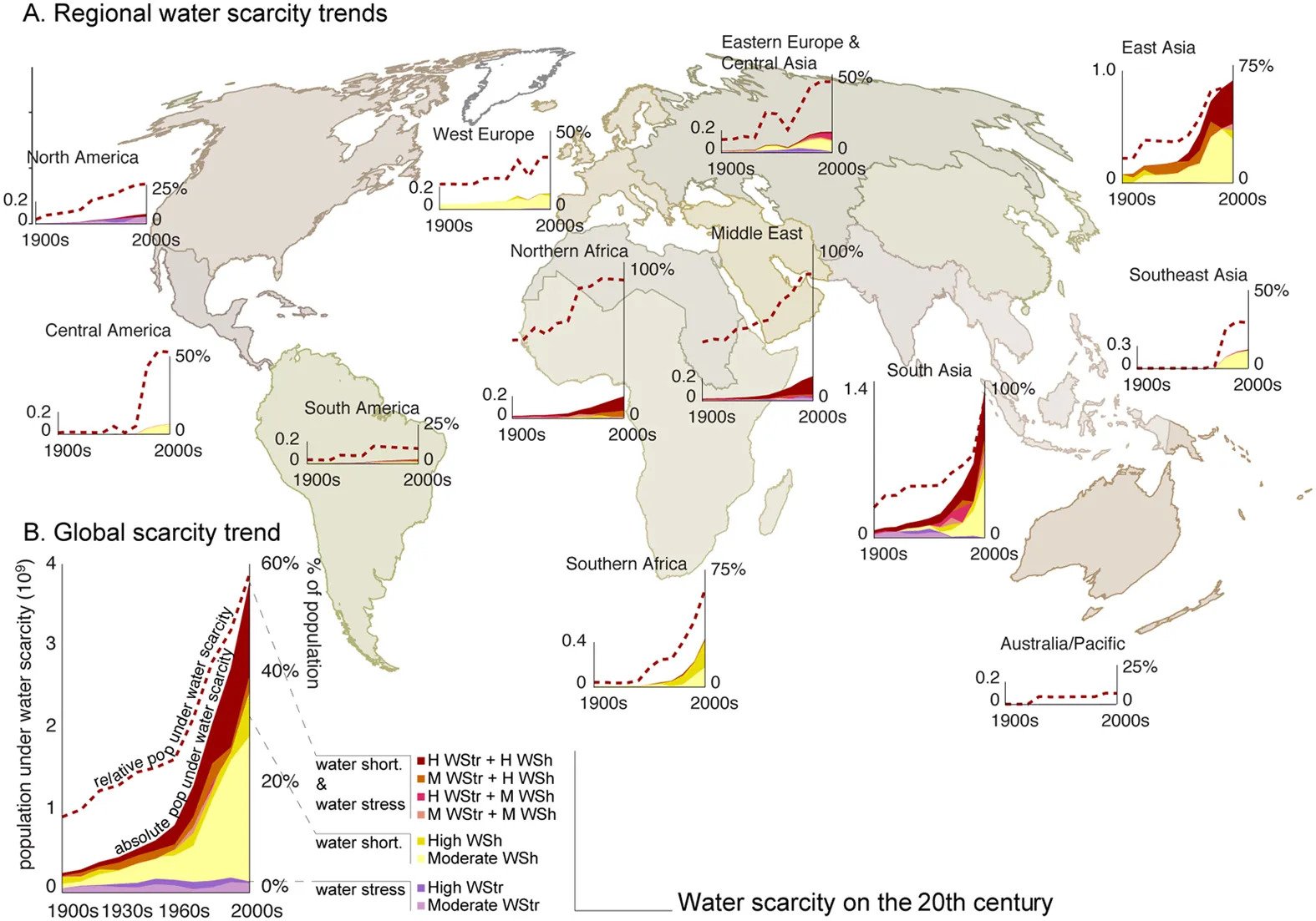
A 2016 article in Nature, The world’s road to water scarcity: shortage and stress in the 20th century and pathways towards sustainability by M. Kummu et. a., looks at water scarcity and shortages (The dotted red line in the graph copied here is the proportion of the population dealing with water scarcity issues. )

Due to increasing population pressure, changing water consumption behavior, and climate change, the challenge of keeping water consumption at sustainable levels is projected to become even more difficult in the near future^5,6.

The increases in population and per capita water consumption resulted in a total water consumption increase from 358 km³ yr⁻¹ in the 1900s to 1500 km³ yr⁻¹ in the 2000s (Fig. 1B).

The article has 6 figures and two data sets available (under electronic supplementary material – right side bar). The richness of the figures makes them useful in a QL or stats course.

A related article from National Geographic, The world’s supply of fresh water is in trouble as mountain ice vanishes by Alejandra Borunda (12/9/2019), discusses the impact of climate change on water supplied by glaciers.

The high mountains cradle more ice and snow in their peaks than exists anywhere else on the planet besides the poles. Over 200,000 glaciers, piles of snow, high-elevation lakes and wetlands: All in all, the high mountains contain about half of all the fresh water humans use.

The high mountains are warming faster than the world’s average; temperatures in the high Himalaya, for example, have crept up nearly 3.6 degrees Fahrenheit (2 degrees Celsius) since the beginning of the century, compared to a planetary average of just about 1.8 degrees F (1 degree C).

“120 million people live along the Indus,” says Immerzeel, “but the Indus plain is like a desert. It’s completely reliant on the water from the thick glaciers above.”

Of the five most important water towers in the world, three are in Asia: the Indus, the Tarim, and the Amu Darya.

The NASA Vital Signs of the Planet article Seal Takes Ocean Heat Transport Data to New Depth by Esprit Smith (12/4/2019) explains (note photo from the article):

But how the current transfers heat, particularly vertically from the top layer of the ocean to the bottom layers and vice versa, is still not fully understood.

Equipped with a specialized sensor reminiscent of a small hat, the seal swam more than 3,000 miles (4,800 kilometers) on a three-month voyage, much of it through the turbulent, eddy-rich waters of the Antarctic Circumpolar Current. The seal made around 80 dives at depths ranging from 550 to 1,090 yards (500 to 1,000 meters) per day during this time. All the while, it collected a continuous stream of data that has provided new insight into how heat moves vertically between ocean layers in this volatile region…

This type of data is available from Marine Mammals Exploring the Oceans Pole to Pole database.

Since 2004, several hundred thousands profiles of temperature and salinity have been collected by instrumented animals. The use of elephant seals has been particularly effective to sample the Southern Ocean and the North Pacific. These hydrographic data have been assembled in quality-controlled databases that can be accessed through this portal.

The Economist’s daily chart Why are Americans’ lives getting shorter? (11/27/19) provides the graphic copied here.

After climbing gradually over the past half century, life expectancy in America reached a plateau in 2010 and then fell for three consecutive years from 2015 to 2017, the latest for which data are available.

Why? Some of it is due to “deaths of despair” with a 386.5% increase in adult drug overdoses from 1999 to 2017. Still:

But the authors note that mortality has increased across 35 causes of death, suggesting that the problem is systemic. Moreover, all racial and ethnic groups have been affected.

OECD life expectancy data.  Starting point for CDC data.

The article by Our World in Data, Pneumonia – no child should die from a disease we can prevent, by Bernadeta Dadonaite (11/12/19) reports:

Every 39 seconds a child dies from pneumonia.

5.4 million children under five years old died in 2017. Pneumonia was the cause of death of one-in-seven of them. . . pneumonia is the leading cause of child mortality globally and has been the leading cause for the past three decades.

What is the distribution of deaths around the world:

As the map shows, children are most likely to die from pneumonia across Sub-Saharan Africa and South Asia. Just 5 countries — India, Nigeria, Pakistan, the Democratic Republic of Congo, and Ethiopia – accounted for more than half of all deaths from childhood pneumonia in 2017.

The disease is therefore most common in places where healthcare infrastructure is lacking and people are least able to afford treatment.

Progress but not enough:

The number of children dying from pneumonia has decreased substantially over the past three decades. In 1990, more than two million children died from pneumonia each year; by 2017 this number had fallen by almost two-thirds.

The post has three graphs with the data.

From the NOAA Global Climate Report – October 2019 page:

The combined global land and ocean surface temperature departure from average for October 2019 was the second highest for October in the 140-year record at 0.98°C (1.76°F) above the 20th century average 14.0°C (57.1°F). This value is just 0.06°C (0.11°F) shy of tying the record warm October set in 2015. The 10 warmest Octobers have occurred since 2003; however, the five warmest Octobers have all occurred since 2015.

This occured with ENSO-neutral conditions during October 2019. Also, January through October for 2019:

The first ten months of 2019 ranked as the second warmest January–October on record, with a combined global land and ocean surface temperature of 0.94°C (1.69°F) above the 20th century average of 14.1°C (57.4°F). This is only 0.09°C (0.16°F) shy of tying the record warm January–October set in 2016.

October time series data from 1880 through 2019 is available here.

The Brookings report Meet the low-wage workforce by Martha Ross and Nicole Bateman (11/7/19) provides demographics of the low-work force by category. The nine categories they use are represented in their chart copied here.  For example, cluster 1 are ages 18-24 are not in school and don’t have a college degree. They are 13% of the low-wage workforce. The post has links to the full report where we learn that this cohort is 51% White, 16% Black, 27% Latino or Hispanic, 2% Asian American, and 4% Other. Of this group, 14% didn’t graduate from high school.

There are regional differences:

Across more than 350 metro areas, the share of workers earning low wages ranges from 30% to 62% of the overall workforce. Low-wage workers are particularly concentrated in smaller places in the southern and western parts of the United States. They make up larger shares of the workforce in places with lower employment rates and that concentrate in agriculture, real estate, and hospitality.

The full report contains a number of data tables.

The St. Louis Fed post Staff Pick: College Education Persists Less for Blacks and Hispanics by Ana Kent (11/12/19 – reposted from Feb) explains:

Educational attainment tells us quite a bit about the types of financial outcomes we should expect a family to have. So does the education of the family’s parents. Unsurprisingly, most people tend to achieve the same level of education as their parents, with college “persisters” (college graduates for whom at least one parent was also a college grad) having the best financial outcomes.

There are racial differences, for example (note: the chart here is population composition – see the table in the article for persistence rates by race):

Blacks had the lowest intergenerational college persistence. If at least one parent had a degree, only 1 in 3 continued to get a college degree themselves.

Intergenerational no-college persistence also showed marked racial differences. Hispanics had the highest no-college persistence, with just under 9 in 10 not achieving a four-year degree if neither parent did.

The post has two graphs and one table.

An article by Fast Company, The first map of America’s food supply chain is mind-boggling by Megan Konar (10/28/19), reports on the paper Food flows between counties in the United States by Xiaowen Lin, et. el. The author of the paper created the network graph of food flow copied here.  From the article:

Overall, there are 9.5 million links between counties on our map.

At 22 million tons of food, Los Angeles County received more food than any other county in 2012, our study year. It also shipped out the most of any county: almost 17 million tons.

Some of the other largest links were inside the counties themselves. This is because of moving food items around for manufacturing within a county—for example, milk gets off a truck at a large depot and is then shipped to a yogurt facility, then the yogurt is moved to a grocery distribution warehouse, all within the same county.

The article has a link to data that created the map. There must be a good graph theory project here.

From the Census Bureau report New Data Show Income Increased in 14 State and 10 of the Largest Metros by Gloria Guzman (9/26/19)

Median household income for the United States and 14 states increased significantly in 2018 from the previous year, according to U.S. Census Bureau data released today.

But,

However, the Gini index of income inequality was significantly higher during the same period for the nation and nine states.

The report has six charts or tables. The full Household Income: 2018 report has tables of data. Historical data including household gini index (table H-4 which includes data by race) is on the Historical Income Tables: Income Inequality page.

Go to the NOAA Climate at a Glance Divisional Mapping page. From the first drop down menu choose a state. Below that a state map appears and now click on a region. If time series data is desired click on the second tab along the top that says time series.  At this point the first drop down menu is to choose a parameter. There are seven choices including average, max, and min temperature as well as precipitation. A time scale can be chosen such as a single month or annual. For example, the graph here created from the site is average annual temperature for the finger lakes region in NYS. Along with a graph, a spreadsheet of the data can be downloaded.