Tag Archives: statistics

How has growth is emigration by region changed?

The Pew Research Center article Latin America, Caribbean no longer world’s fastest growing source of international migrants by  Luis Noe-Bustamante and Mark Hugo Lopez (1/25/19) provides an overview emigration changes by region. The graph copied here shows how the growth in emigration from Latin America and the Caribbean has drooped from 58% from 1990-2000 to 7% for 2010-2017, which is slower than thew worldwide growth rate of 17%. On the other hand, 

Even though the percentage growth of the emigrant population from Latin American-Caribbean nations has slowed, the region is still a large source of emigrants. About 37 million people from the region lived outside their country of birth in 2017, up from 35 million in 2010 and accounting for nearly 15% of the world’s more than 250 million international migrants in 2017. The Asia-Pacific region is the source of the world’s largest emigrant population (85 million), as well as the largest share of the global total (33%).

The article includes three other charts, a table of data, and a methodology section with sources.

More than half the U.S. population lives in what percent of counties?

The answer is the title of the Census Bureau post More Than Half of U.S. Population in 4.6 Percent of Counties by Haya el Nasser (10/24/18). The map copied here shows the counties.

At the county level, the geographic distribution of the estimated 325.2 million people in the United States clearly distinguishes two main areas where people live: “big” counties and “small” counties.

More than half of all residents live in just 143 big counties (in terms of the number of residents), according to an analysis of U.S. Census Bureau county estimates. That means less than half of the population is spread out across the remaining 2,999 small counties.

The post has a short video with more information. For instance the average population density of big counties is 926 people per square mile and only 48 people per square mile for small counties. Small counties are almost 75% non-Hispanic white, while big counties are under 50% non-Hispanic white.

There is also a notable difference in the rate of growth. “Big-county America is growing nearly twice as fast as small-county America,” Sink said. “They’re not only getting bigger but increasingly more diverse.” Thus, if current trends continue, it’s likely that the divide between big and small will continue to become more pronounced in the future.

The post has  another map and some useful tables which include the distribution of small and large counties.

What are the demographics of 6- 21 year olds?

The Pew article Early Benchmarks Show ‘Post-Millennials’ on Track to Be Most Diverse, Best-Educated Generation Yet – A demographic portrait of today’s 6- to 21-year-olds by Richard Fry and Kim Parker (11/15/18)  provides demographic information comparing early boomers, gen xers, millennials, and post millennials.  For example, the graph copied here shows the changes in racial groups across the four generations. The trend toward cities contiues:

The geography and mobility of post-Millennials differ from earlier generations. Reflecting broader national trends, post-Millennials overwhelmingly reside in metropolitan as opposed to rural areas. Only 13% of post-Millennials are in rural areas, compared with 18% of Millennials in 2002. By comparison, 23% of Gen Xers lived in rural areas when they were ages 6 to 21, as did 36% of early Boomers.

The distribution of racial groups by region differs (also see the second graph):

In the West, post-Millennials are just as likely to be Hispanic as non-Hispanic white (both 40%). This stands in contrast to older generations. Among those residing in the West, 45% of Millennials, 50% of Gen Xers and 64% of Boomers are non-Hispanic white. Minority representation among post-Millennials is lowest in the Midwest, where roughly a third (32%) of 6- to 21-year-olds are racial or ethnic minorities.

The Pew report includes 12 charts and a methods section with links to the data.

How effective is gerrymandering?

The article in Isthmus No contest – Dems sweep statewide offices in midterms but remain underrepresented in Assembly by Dylan Brogan (11/15/18) presents the graphic copied here. In short the dems won all races in terms of the popular vote but control only 36 of the 99 seats in the assembly.

“The biggest obstacle remains gerrymandering. There are only a handful of districts that are remotely competitive. That’s why a district court ruled the [legislative] maps unconstitutional and why we still have a case before that court,” says Hintz, referring to Gill v. Whitford which the U.S. Supreme Court sent back to the lower federal court for reargument. “Gerrymandering doesn’t just have an impact on the outcome. It has an impact on being able to recruit candidates. There aren’t a lot of people willing to run when they know they don’t have a shot.”

Three sources to learn more about the mathematics of gerrymandering: The Math Behind Gerrymandering and Wasted Votes by Patrick Honner (10/12/17), Countermanding Gerrymandering with a short podcast with Moon Duchin, and Detecting Gerrymandering with Mathematics by Lakshmi Chandrasekaran (8/2/18) .

Our recent post How do you tell a story with data and maps – Beto vs Cruz? (11/15/18) notes how to obtain election data. The chart made here for WI can be done for other states as a stats project.

How do you tell a story with data and maps – Beto vs Cruz?

FiveThirtyEight has an excellent article on the 2018 senate race and the possible implications for future elections. The article, What Really Happened In Texas by Kirk Goldsberry (11/14/18) analyzes voting patterns by county and compares 2014 to 2018.  Their graph copied here is the fourth in a series of maps and mostly summarizes the previous maps.

Cruz won by 220,000 votes last week. But in Harris County alone, 500,000 more people voted in the 2018 midterms than had voted in 2014. In Dallas County, 300,000 more people voted than in the last midterms, and in Travis, Bexar and Tarrant counties, 200,000 more people voted.

Indeed, aside from some noteworthy increase in voter numbers in suburban Dallas, the biggest white circles on the map above tend to hover over Beto country. Meanwhile, the darkest red counties — the places that carried Cruz back to Washington — have exhibited very little, if any, change in the number of votes cast compared to 2014. Those areas may be staunchly red, but they’re also staunchly stagnant too. O’Rourke almost won in 2018 by taking roughly 60 percent of the vote in the big five counties. This map suggests that if Democrats can repeat that feat as these places continue to grow, that may be all they need to turn Texas blue.

The data for their analysis comes from the Texas Secretary of State election results.  The 2014 data is available by following the Historical Election Results (1992-current) link. The 2018 data is available through a link along the top. This is a stats project in the making (do this for you home state). The article can also  be used in a QL course.

How does the digital divide impact secondary education for different groups?

The Pew Research Center article Nearly one-in-five teens can’t always finish their homework because of the digital divide by Monica Anderson and Andrew Perrin (10/26/18) provides insights on how lacking access to the internet impacts the ability to complete homework.  Their chart (copied here) gives the percent of school-age children by race and income without high-speed internet.  A second chart provides the results of survey about how this impacts homework. In particular,

One-quarter of black teens say they are at least sometimes unable to complete their homework due to a lack of digital access, including 13% who say this happens to them often. Just 4% of white teens and 6% of Hispanic teens say this often happens to them. (There were not enough Asian respondents in this survey sample to be broken out into a separate analysis.)

The article includes a link at the bottom for results and methodology. This includes sample sizes making this article particularly useful for statistics courses.

Who misses school the most?

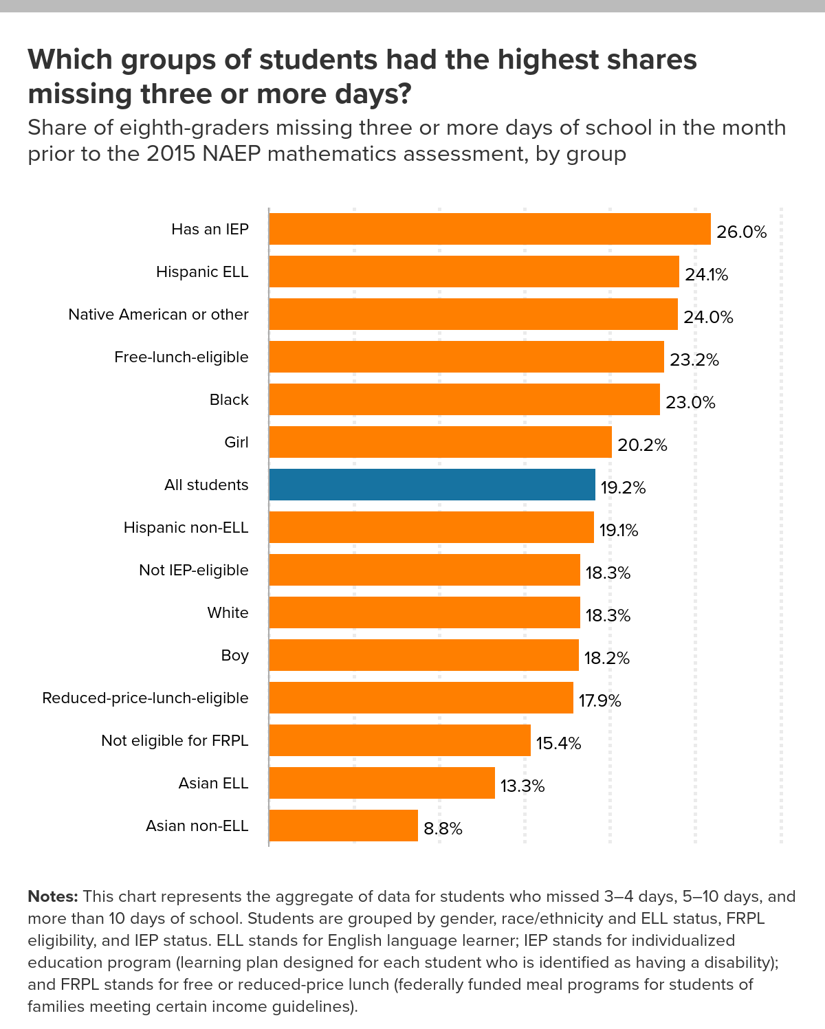
The EPI article,  Student absenteeism – Who misses school and how missing school matters for performance by Emma García and Elaine Weiss (9/25/18) provides a detailed account of absenteeism based on race and gender.  For example, their chart here is the percent of students that missed three or more days in the month prior to the 2015 NAEP mathematics assessment. There are noticeable differences. For instance, the percentage of Black, White, and Asian (non ELL) that missed three or more days in the month is 23%, 18.3%, and 8.8% respectively.

Why does this matter?

In general, the more frequently children missed school, the worse their performance. Relative to students who didn’t miss any school, those who missed some school (1–2 school days) accrued, on average, an educationally small, though statistically significant, disadvantage of about 0.10 standard deviations (SD) in math scores (Figure D and Appendix Table 1, first row). Students who missed more school experienced much larger declines in performance. Those who missed 3–4 days or 5–10 days scored, respectively, 0.29 and 0.39 standard deviations below students who missed no school. As expected, the harm to performance was much greater for students who were absent half or more of the month. Students who missed more than 10 days of school scored nearly two-thirds (0.64) of a standard deviation below students who did not miss any school. All of the gaps are statistically significant, and together they identify a structural source of academic disadvantage.

These results “… identify the distinct association between absenteeism and performance, net of other factors that are known to influence performance?”  The article has 12 graphs or charts, with data available for each, including one that reports p-values.
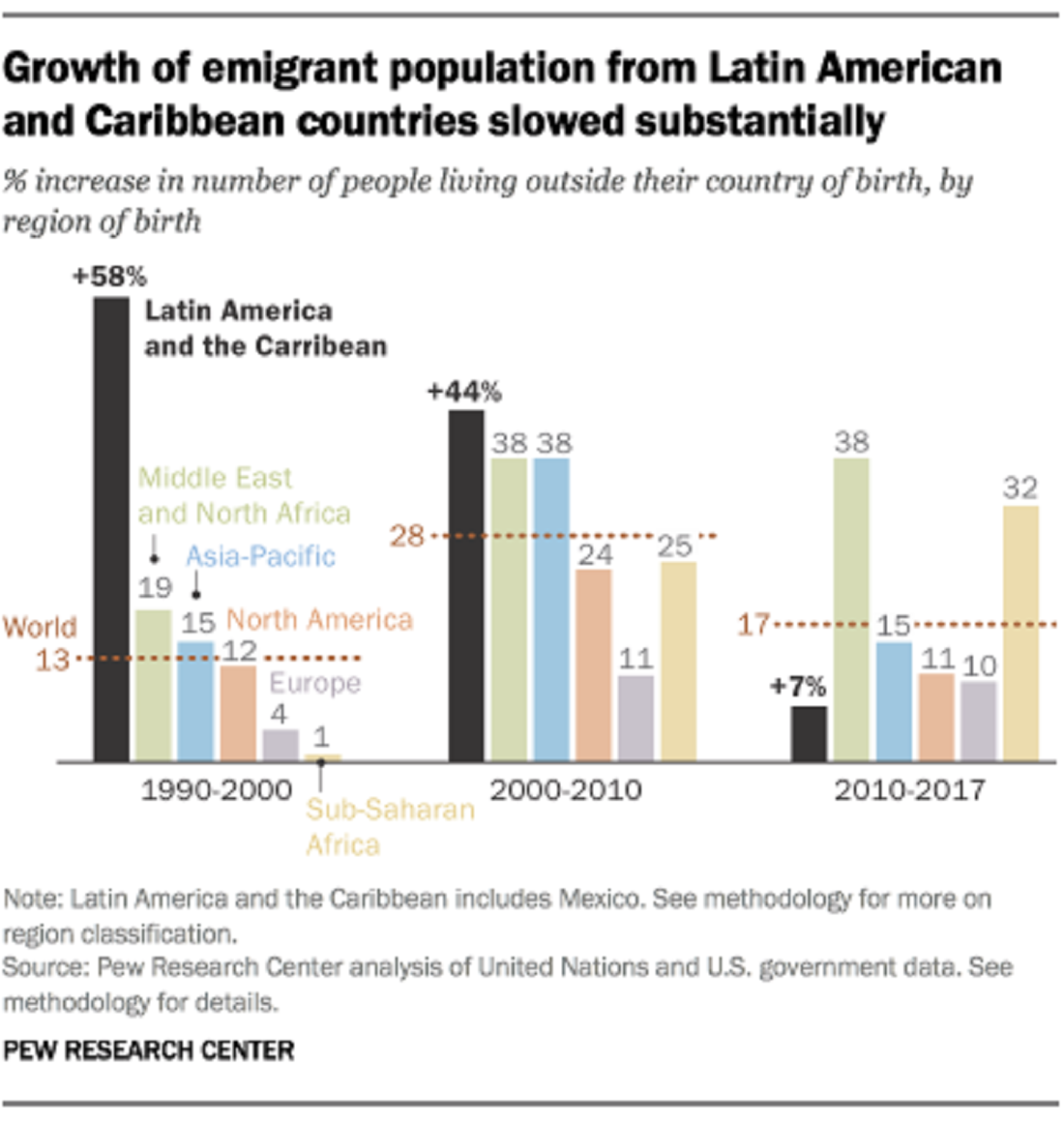
How much have fall temperatures risen?

According to the Climate Central post, Fall Warming Trends Across the U.S. (9/5/18), the average fall temperature for the U.S. has risen nearly 3°F since 1970 (see their graph copied here).  Why does this matter:

Insects linger longer into the fall when the first freeze of the season comes later in the year. A new study from the Universities of Washington and Colorado indicates that for every degree (Celsius) of warming, global yields of corn, rice, and wheat would decline 10 to 25 percent from the increase in insects. Those losses are expected to be worst in North America and Europe.

The article has a drop down menu to select cities across the U.S. to see a graph similar to the one copied here for the selected city.  They don’t post the data that was used to create the graphs but they do explain their data sources under methodology.

A statistics project could have students create this graph for their hometown.  One way to obtain the data was noted in our post, What do we know about nighttime minimum temperatures?: Go to  NOAA’s Local Climatological Data Map. Click on the wrench under Layers. Use the rectangle tool to select your local weather station. Check off the station and Add to Cart. Follow the direction from their being sure to select csv file. You will get an email link for the data within a day.  Note: You are limited in the size of the data to ten year periods. You will need to do this more than once to get the full data set available for your station.


How much do countries spend on education?

The answer to the question depends on how it is measured.  The post  in statista, The Countries Spending the Most on Education by Martin Armstrong (9/12/2018) reports spending as a share of gross domestic product for primary, second and post-secondary non-tertiary education as well as tertiary education.  By this measure Norway spends the most. But, if the measure used is expenditure per student as a share of GDP per capita, the high spender is (south) Korea (Norway is fifth). Our graph here is a scatter plot of the two measures by country.

The data is from OECD.Stat. Go to Education and Training, Education at a Glance, Financial resources invested in education, Education finance indicators, and finally Expenditure per student as share of GDP per capita.  Under indicator at the top of the spreadsheet the measure can be changed.  Definitions of measures can be found in the OECD Handbook for Internationally Comparative Education Statistics (page 99).

Download the csv file and R-script used here.

What do we know about plastics?

The Our World in Data article Plastic Pollution by Hannah Ritchie and Max Roser (Sept 2018) is a detailed summary of plastics with 20 charts.  For example, one of the charts is a time series of plastic production (downloaded and posted here) showing that, in 2015, the world produced 381 million tons of plastic. In the same year, only 20% of the plastic was recycled (second chart in the article).  There is information on plastic waste generation.

Packaging, for example, has a very short ‘in-use’ lifetime (typically around 6 months or less). This is in contrast to building and construction, where plastic use has a mean lifetime of 35 years.7 Packaging is therefore the dominant generator of plastic waste, responsible for almost half of the global total.

Who produces the most plastic waste?

… we see the per capita rate of plastic waste generation, measured in kilograms per person per day. Here we see differences of around an order of magnitude: daily per capita plastic waste across the highest countries – Kuwait, Guyana, Germany, Netherlands, Ireland, the United States – is more than ten times higher than across many countries such as India, Tanzania, Mozambique and Bangladesh.

As always with Our World in Data, the data associated with each graph is downloadable.