What is the story of suicides in the U.S.?

The article in the Conversation, Why is suicide on the rise in the US – but falling in most of Europe? by Steven Stack (6/28/18), tries to get at the story. The first chart (copied here), clearly shows that the suicide rate rose from 199-2015 overall and considerably more for the 45-54 age group (stats regression problem here).  There is a second chart showing changes in suicide rates in Western European countries:

However, suicide rates in other developed nations have generally fallen. According to the World Health Organization, suicide rates fell in 12 of 13 Western European between 2000 and 2012. Generally, this drop was 20 percent or more. For example, in Austria the suicide rate dropped from 16.4 to 11.5, or a decline of 29.7 percent.

The obvious question is why?

There has been little systematic research explaining the rise in American suicide compared to declining European rates. In my view as a researcher who studies the social risk of suicide, two social factors have contributed: the weakening of the social safety net and increasing income inequality.

The article has two more charts showing that the U.S. is low on Social Welfare Expenditures as a percent of GDP and is high on inequality. In all instances the data is available for download and there are links to the original sources.

How hot has it been this week?

Simulation of maximum temperatures on July 3 from American (GFS) weather model at two meters above the ground. (University of Maine Climate Reanalyzer)

The Washington Post article, Red-hot planet: All-time heat records have been set all over the world during the past week by Jason Samenow (7/5/18), provides a nice overview of the record setting heat during this past week (map posted here copied from the article).  In North America:

Montreal recorded its highest temperature in recorded history, dating back 147 years, of 97.9 degrees (36.6 Celsius) on July 2. The city also posted its most extreme midnight combination of heat and humidity.

Ottawa posted its most extreme combination of heat and humidity on July 1.

In Europe:

Excessive heat torched the British Isles late last week. The stifling heat caused roads and roofs to buckle, the Weather Channel reported, and resulted in multiple all-time record highs:

In the Middle East:

As we reportedQuriyat, Oman, posted the world’s hottest low temperature ever recorded on June 28: 109 degrees (42.6 Celsius).

Maps of temperature anomalies can be created for various time periods from NASA’s GISS Surface Temperature Analysis page. June isn’t available yet but it will be before long.  Monthly Global Climate reports are available from NOAA. June isn’t available yet, but here are two highlight from May:

The contiguous U.S. May 2018 temperature was 2.89°C (5.2°F) above the 20th century average and the highest May temperature since national records began in 1895. This value exceeds the previous record set in 1934 by +0.4°C (+0.7°F).

Europe had its warmest May since continental records began in 1910 at +2.76°C (4.97°F), surpassing the previous record set in 2003 by +0.92°C (+1.66°F). May 2018 marks the first time in May that the continental temperature departure from average is 2.0°C (3.6°F) or higher.

Do we disagree with factual statements that we think are opinions?

The Pew Research Center’s article Distinguishing Between Factual and Opinion Statements in the News by Amy Mitchell, Jeffrey Gottfried, Michael Barthel, and Nami Sumida (6/18/18) addresses this question and more.

A new Pew Research Center survey of 5,035 U.S. adults examines a basic step in that process: whether members of the public can recognize news as factual – something that’s capable of being proved or disproved by objective evidence – or as an opinion that reflects the beliefs and values of whoever expressed it.

We will focus on section 4 Americans overwhelmingly see statements they think are factual as accurate, mostly disagree with factual statements they incorrectly label as opinions. Odds are that a person who identifies a factual statement as opinion will also disagree with the statement (see table copied here).  For example,  41% of those surveyed said that Spending on Social Security, Medicare, and Medicaid make up the largest portion of the U.S. federal budget was an opinion and of those 82% disagreed with the statement.

This is an excellent article for a QL or Stats course as it is rich with data, graphs, and charts. You can also discuss why 41% of those surveyed thought a statement that is measurable (How much of the Federal budget goes to social security, medicare, and medicaid?) was an opinion.  The article also includes detailed information on their methodology and detailed tables of data.


How much are 30 year temperature averages increasing?

Changes in 30 year temperature averages depend on where you live, but Climate Central’s New Normal: Temperatures Are Trending Up Across U.S.  (3/16/18) has graphs for major cities across the U.S. The one here is for the U.S.

Normal temperatures, generally defined to be the 30-year average at a location, are trending up across most of the U.S. Since 1980, the average continental U.S. temperature has risen 1.4°F.

This is a change in the 30 year average so that the value for 2017 is the average from 1988-2017. In other words, the climate is changing.  A nice primer on the difference between weather and climate can be found at the NSIDC Climate vs Weather page:

Weather is the day-to-day state of the atmosphere, and its short-term variation in minutes to weeks. People generally think of weather as the combination of temperature, humidity, precipitation, cloudiness, visibility, and wind. We talk about changes in weather in terms of the near future: “How hot is it right now?” “What will it be like today?” and “Will we get a snowstorm this week?”

Climate is the weather of a place averaged over a period of time, often 30 years. Climate information includes the statistical weather information that tells us about the normal weather, as well as the range of weather extremes for a location.

The Climate Central post has a drop down menu and you can choose the graph for the city closest to you to see how much your climate has changed.  They don’t post the data that was used to create the graphs, but you can find the data for a location near you. Try starting with this NOAA map (look for a future post on using this portal for local data). This could be a great stats project for students.
 

How has forest area changed around the world?

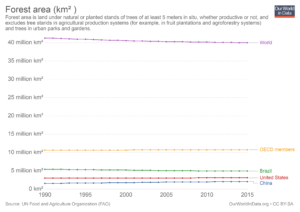
Our World in Data answers the question with an interactive chart of forest area by country and regions from 1990 to 2015.  In that time period the world has lost 1.29 million square km of forest area (41.28 to 39.99). On the other hand, the U.S. and China both increased forest area by 0.08 (3.02 to 3.1) and 0.51 (1.57 to 2.08 – a 32% increase) msk respectively, while Brazil lost 0.53 msk (5.47 to 4.94).  As always with Our World in Data, you can download charts (as we did here with our selected countries and regions) and the data.

Why are forest important?  The USDA Forest Service Ecosystem Services page is a starting point to learn more.

Healthy forest ecosystems are ecological life-support systems. Forests provide a full suite of goods and services that are vital to human health and livelihood, natural assets we call ecosystem services.

Many of these goods and services are traditionally viewed as free benefits to society, or “public goods” – wildlife habitat and diversity, watershed services, carbon storage, and scenic landscapes, for example. Lacking a formal market, these natural assets are traditionally absent from society’s balance sheet; their critical contributions are often overlooked in public, corporate, and individual decision-making.

In particular, forests play a role in climate change. Learn more and some basic science from the FAO Forests and climate change Carbon and the greenhouse effect

Is math involved in modeling forest? Yes, The Smithsonian’s National Zoo & Conservation Biology Institute article Using Mathematical Models to Save Forests (3/27/2018) provides one example:

In collaboration with partners from universities in the western U.S., South America and New Zealand, Smithsonian scientists have developed a mathematical model to help understand why certain landscapes are especially vulnerable to losing their forests and the species that rely on them, while others are more resilient.

What economic impacts does some college education have on men?

The article in the Conversation 22 percent of men without college don’t have jobs. Here’s why they’re being left behind. by Erin Wolcott (6/7/2018) makes two points:

But the unemployment rate doesn’t tell the full story because it only includes people actively looking for work. People who report not having looked for work in the previous four weeks are completely left out of this number. The employment rate, which is the share who are actually employed, captures the full picture.

And the numbers are stark. Back in the 1950s, there was no education-based gap in employment. About 90 percent of men aged 25-54 – regardless of whether they went to college – were employed.

The Great Recession was particularly painful for men without any college. By 2010, only 74 percent had a job, compared with 87 percent of those with a year or more of college.

By 2016, from the graph here copied from the article, the gap was 90% vs 78%. For the second point:

The gap extends to the wages of those who actually had jobs as well. As recently as 1980, real hourly wages for the two groups were nearly identical at about US$13. In 2015, men with at least a little college saw their wages soar 65 percent to over $22 an hour. Meanwhile, pay for those who never attended plunged by almost half to less than $8.

The article has another graph for wages. Both graphs are interactive and contain links to download the data. Read the article.

How fast is Antarctica melting (and a quick calculus project)?

A recent NYT article, Antarctica Is Melting Three Times as Fast as a Decade Ago by Kendra Pierre-Louis (6/13/2018), states clearly that Antarctica is melting, well, three times faster than a decade ago, which is a rate of change statement. Rapid melting should cause some concern since:

Between 60 and 90 percent of the world’s fresh water is frozen in the ice sheets of Antarctica, a continent roughly the size of the United States and Mexico combined. If all that ice melted, it would be enough to raise the world’s sea levels by roughly 200 feet.

Any calculus student can roughly check the melting statement.  Antarctica ice data is available at NASA’s Vital Signs of the Planet Ice Sheets page. There you can download change in Antarctica ice sheet data since 2002. (Note: The NYT article has a graph going back to 1992, but ends in 2017 as does the NASA data.) A quick scatter plot and a regression line shows that the change is not linear and the data set is concave down. (The graph here is the NASA data and produces in R – the Calculus Projects page now has some R scripts for those interested.)  Now, a quadratic fit to the data followed by a derivative yields that in 2007 the Antarctica was losing 95 gigatonnes of ice per year and in 2017 it was 195.6 gigatonnes per year. Even with this quick simple method melting has more than doubled from 2007 to 2017. The NYT article states:

While that won’t happen overnight, Antarctica is indeed melting, and a study published Wednesday in the journal Nature shows that the melting is speeding up.

This is an excellent sentence to analyze from a calculus perspective. Given that the current trend in the data is not linear and at least about quadratic, then melting is going to increase each year.  On the other hand, maybe they are trying to suggest that melting is increasing more than expected under past trends, for example the fit to the data is more cubic than quadratic. In other words, is the derivative of ice loss linear or something else? If everyone knew calculus the changes in the rate of ice loss could be stated precisely.

How much are the oceans warming?

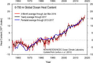
A year ago Climate Central posted the article Oceans Are Heating Up with a graph of sea surface temperature anomalies while providing context on issues of ocean warming:

 93 percent of the excess heat absorbed by the climate system goes into our oceans, creating major consequences. While more extreme storms and rising sea levels are some of the impacts of warmer oceans, rising CO2 levels and the resulting warmer oceans are impacting ocean health itself. The most well­ known effects are coral bleaching and ocean acidification, but an emerging issue is the decreasing oxygen levels in the warming waters.

The graph here is from NOAA’s Global Ocean Heat and Salt Content page. There you will find numerous updated graphs related to ocean heat content.  For related data go to NOAA’s Basin time series of heat content page to find about 50 time series on ocean heat.

For context on units, a person at rest typically generates about 60 joules of heat per minute while the graph here has y-axis units of 10^22 Joules.

What are the symptoms of inequality?

The Guardian article, Trump’s ‘cruel’ measures pushing US inequality to dangerous level – UN warns by Ed Pilkington (6/1/18) lists some symptoms two of which are:

Americans now live shorter and sicker lives than citizens of other rich democracies;

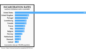
The US incarceration rate remains the highest in the world;

The article lacks some data, which we provide here. It is true that incarceration rates in the U.S. are shockingly the highest in the world, see the chart here from the Prison Policy Initiative’s States of Incarceration: The Global Context 2018. But, this isn’t much different than in 2016 as compared to Prison Policy Initiative’s States of Incarceration: The Global Context 2016 report. Both PPI pages have links to the data sets at the bottom as well as other graphs.

As for U.S. life expectancy Our World in Data has an interactive life expectancy graph.  The last year for this graph is 2015, but by that time the U.S. already had a lower life expectancy than other wealthy countries. This graph allows us to choose other countries, has a map version, and a link to download the data.

In short, the symptoms of inequality stated in the Guardian article are not new (at least the two we focused on here), although they may be getting worse. The article is worth wording as well as the PPI report. Also explore the Our World in Data life expectancy graph. There is data and context to connect all this to stats or QL courses.


Do people in poverty work?

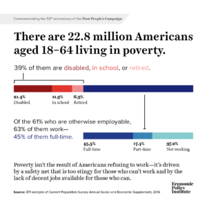
The EPI article, 50 years after the Poor People’s Campaign poverty persists because of a stingy safety net and a dysfunctional labor market by Elise Gould and Jessica Schieder (5/24/2018), answers the question with a graph (reposted here) and this:

The bottom bar shows us that, among those working-age individuals who are otherwise employable, 63 percent are working and 45.5 percent are working full time. An additional 37.2 percent are not working, but this share includes 1.6 million people living below the poverty line who are actively seeking a job. The data make it clear that millions of people who are active participants in the labor market are unable to make ends meet, either due to insufficient hours or low wages.