One more post from the Manhattan Institute’s* Breaking Down the 2020 Homicide Spike by Christos A. Makridis and Robert VerBruggen (5/18/2022). We first note:
Homicides went up throughout the country, and for every major demographic group, in 2020, but they did not rise for everyone equally, as is clear when we break down the numbers by race, age, sex, urbanicity, and region of the country.
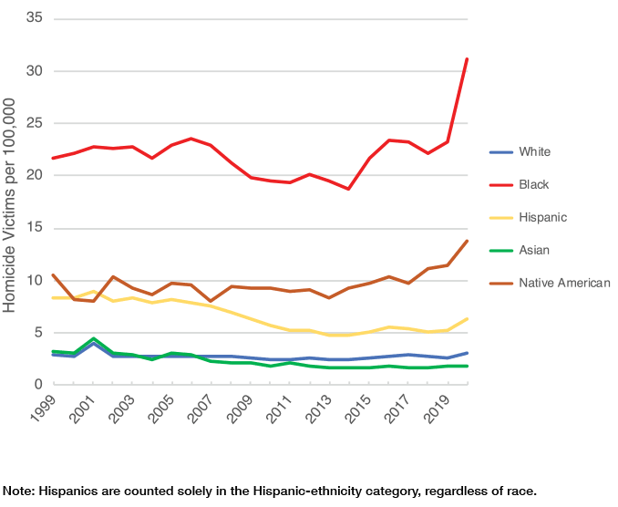
Related to figure 3 (copied here) we have this, which is excellent QL material:
The racial and ethnic breakdown is perhaps most striking in this regard. Proportionally, homicide rates rose by about 34% for black Americans and about 19% percent for non-Hispanic whites: a notable, but not extreme, gap (Figure 3). But since the black homicide rate was already many times higher than the white one, this translated into 8 additional black deaths for every 100,000 population—an increase similar to the total homicide rate for the country as a whole—while the death rate for whites rose by only 0.5 per 100,000. (Recall that these numbers pertain to the homicide victims, not the killers, though American homicide is overwhelmingly intraracial.)
There is a lot to discuss in this article as well as ample quantitative literacy material. There is a discussion of methods and the CDC data they use is easy enough to locate.
* (This is the same note from Monday’s Post) Yes, MI has a clear political leaning but that doesn’t make their work incorrect. Their data and methods are sound here and this should be engaged not ignored. If someone thinks something is incorrect then let me know.
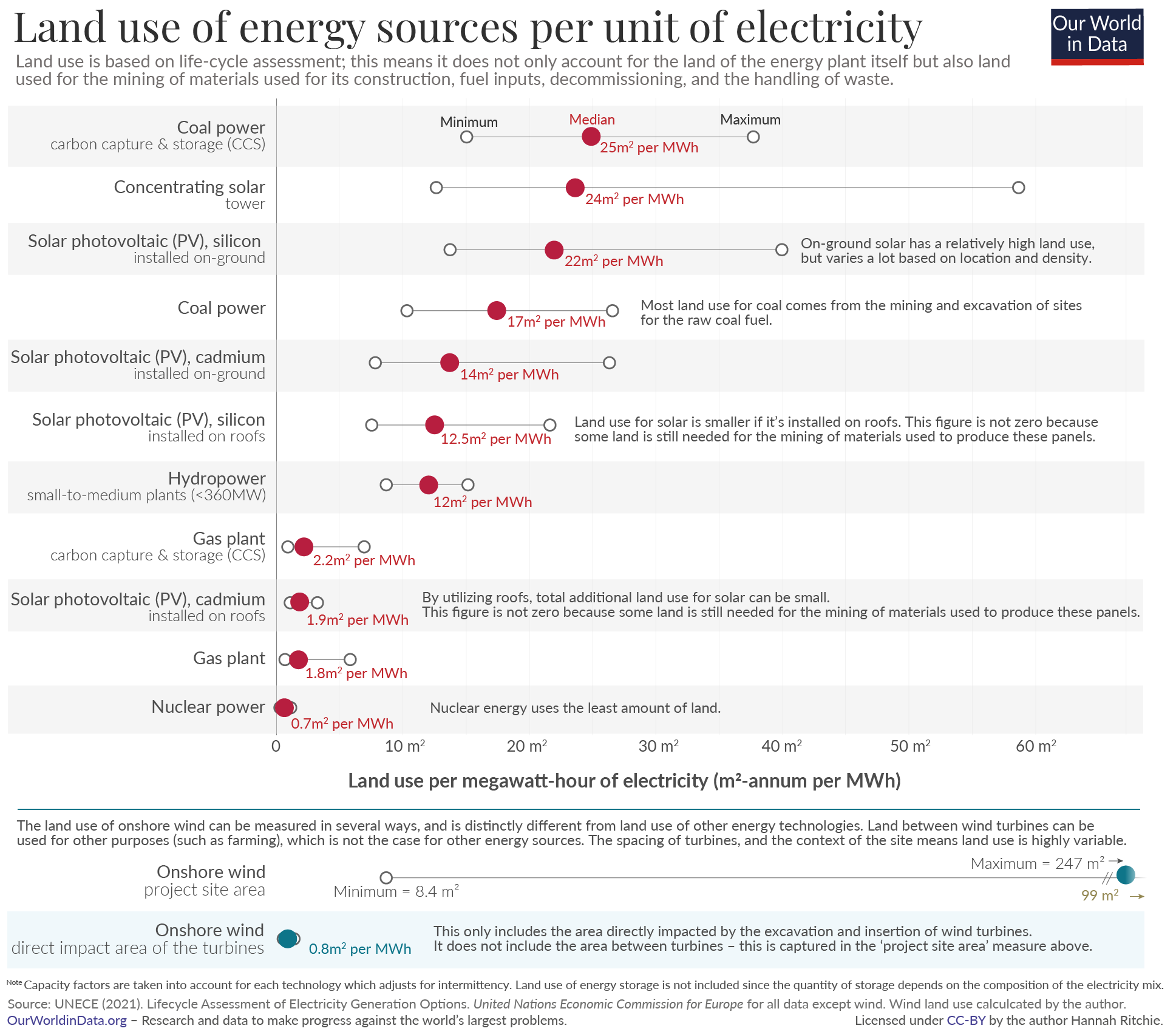 The Our World in Data article How does the land use of different electricity sources compare? by Hannah Ritchie (6/16/2022) looks to answer this question. Here is what they consider: