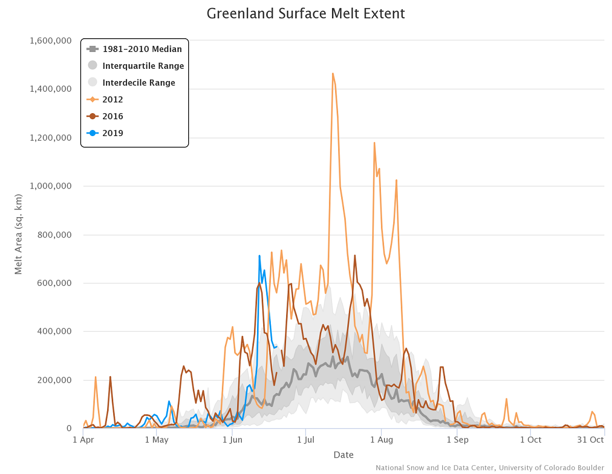
Tag Archives: charts and graphs

The EIA has a new portal for state energy information. The new portal is introduced in the post New EIA Product Expands Access to State and Regional Energy Information by Stacy Angel and Pauline George (5/16/19).

EIA’s new State Energy Portal provides greater access to more state-level U.S. energy data with interactive, customizable views of more than 150 charts, tables, and maps. Infographics show the overall energy context for the states; state rankings provide a way to compare states. Users can download charts and embed them in their websites.

For example, the chart here is from the new portal. It is natural gas consumption by sector in New York from 2014 through Feb. of  2019. Notice the relationship between residential and electric power. Quiz question: Why does residential and electric power peak at opposite time of the year? The choices for this individual data set included a time range dating back to 1990, stacked bar chart, or table. The data is also available. Choose a state, an energy product, and explore.

The yearly EPI report on economic prospects for young college grads Class of 2019 College Edition by Elise Gould, Zane Makhiber, and Julia Wolfe (5/14/19) is now available. The report has 19 key finding and 10 graphs with available data. A few highlights:

Women make up half of 21- to 24-year-olds but well over half (57.4 percent) of young college degree holders.

One out of every 20 young college graduates is unemployed, a higher rate than in 2000, when only one in 25 was.

After falling in the aftermath of the Great Recession, wages for young college graduates have been growing steadily since 2014 and have (just barely) surpassed the 2000 benchmark; however, nearly two decades of wage growth for young college graduates have been lost.

Related Post: What are the prospects for new college grads? (5/21/18)

The Weather Channel article It’s the Year 2100 and Everyone’s Moving to Duluth by Neil Katz (4/16/19) notes

In a climate-changed future many people, says Keenan, “are looking for affordability, accessibility and actually qualitatively some degree of environmental amenities, which we believe Duluth, Lake Superior, and that part of northeast Minnesota, among other places may offer.”

Huttner is right to point out that winter weather in Duluth remains brutally cold, snowy and difficult. But it is changing, and it’s changing faster than many other places. Winters are now five degrees warmer than they were in 1970, according to NOAA data analyzed by Climate Central.

The Weather Channel isn’t the only one praising Duluth as a future place to live. The NYT article Want to Escape Global Warming? These Cities Promise Cool Relief by Kendra Pierre-Louis (4/15/19) lists Duluth and Buffalo as cities of the future (Note: Both articles quote Keenan, a lecturer at Harvard University Graduate School of Design). The Weather Channel article has a couple of nice charts (such as the one copied here) and both are a starting point for conversations about adapting to climate change.

PS On a personal note, I lived in the Twin Ports (Duluth MN and Superior WI) for a couple of years around 2000. Beautiful place.

This recent video (3/29/19) by Robert Rohde shows how temperature distributions have changed. Each year the graph is a distribution of temperature anomalies.  As noted “This essentially the same data that was previous shown as an animated map:”  https://www.youtube.com/watch?v=JObGveVUz7k  The video here is useful in any statistics or QL course and the two videos together provide an illustration of how to display data. The data is from Berkeley Earth.

The melting season for Arctic Sea Ice has started with a quick drop in ice. The total ice is at a record low for this time of year (orange line in chart). But, how this plays out throughout the melting seasons is hard to predict based solely on past seasons. For instance, 2012 is the year of the record low (dashed line), but numerous seasons have been lower than 2012 at this time of year (2016 – yellow, 2015 – green, 2007 – blue shown here).  Arctic Sea Ice extent is updated daily on the Charctic Interactive Sea Ice Graph by NSIDC. This graph allows the user to select years, download the image, and choose between Arctic and Antarctic ice extent. NSIDC posts the data and there is a project on both the Calculus and Statistics page using this data, as well as an interactive graph.

Pew has an interactive graph on their Remittance flows worldwide in 2017 page where you can select a country and either outgoing or incoming. The result is get a map of how much money was sent to other countries or came into the country. For example, the graph here is for money sent from the U.S. to other countries. Along with the map, a table of data is updated to match the selection on the map.  A related Pew article, Immigrants sent a record amount of money home to sub-Saharan African countries in 2017 by Abby Budiman and Phillip Connor (4/3/19), highlights this data.

Money sent by immigrants to their home countries in sub-Saharan Africa reached a record $41 billion in 2017. This represents a 10% jump in remittances from the previous year, the largest annual growth for any world region, according to a Pew Research Center analysis of World Bank data.

Worldwide, immigrants sent a record $625 billion (in 2018 U.S. dollars) back to their home countries in 2017, a 7% increase from the previous year.

There are three more interactive graphs on the Interactive Graphs page for a total of five.  One is Arctic Sea Ice extent by year for the months of March (high month), June, September (low month), and December, along with regression lines and residual plots (snapshot here). The other two represent the expected years to live at a given age. One of these is by race and gender, while the other is all females and males. Both graphs include a regression line and residual plot. The purpose of these graphs is to not only be interesting and informative, but to also be useful as classroom resource for projects or exercises.

The Council of Graduate Schools (CGS) report, Graduate Enrollment and Degrees 2007 to 2017 (Oct 2018) provides data on enrollment and degrees in graduate school by gender and race.  For example, the graph here is Figure 2 in their report and provides enrollment data by field of study and  gender.  In the aggregate they note:

Academic year 2016-17 marked the eighth consecutive year in which women earned the majority of degrees awarded at the doctoral level. Women earned 64.0% of graduate certificates awarded in 2016-17, 57.3% of master’s degrees, and 53.0% of doctorates.

The report contains a number of graphs and data tables with various  demographic information (race, gender, international). For example,

Among first-time U.S. citizens and permanent resident graduate students in the Fall of 2017, about 23.9% were underrepresented minorities, including American Indian/Alaska Native (0.5%), Black/African American (11.9%), Native Hawaiian/Other Pacific Islander (0.2%), and Hispanic/Latino (11.3%) (Table B.11).

A summary page of the report, First-Time Enrollment Holds Steady – Application Counts Slightly Decline at U.S. Graduate Schools, also has a link to the full pdf report.

EPI has released its report: State of Working America Wages 2018, Wage inequality marches on – and is even threatening data reliability by Elise Gould (2/20/19). The report includes 19 tables and charts. The data and charts are easily downloaded, such as the chart here. The report is thorough and anyone reading it will likely be surprised about something.  A few selection from the report:

From 2017 to 2018, men at the 95th percentile saw large wage gains, while those at the middle and very bottom of their wage distribution experienced downright wage losses.

The gender wage gap at the 10th percentile remains the smallest across the wage distribution and it has narrowed since 2000; it is currently at 5.9 percent. The regression-adjusted average gender wage gap narrowed slightly from 2000 to 2018 and is currently at 22.6 percent.

In both comparison periods, both men and women at the 10th percentile saw greater wage growth in states with minimum wage changes versus those without.

Over the last 18 years, wage growth for white and Hispanic workers has been about four times faster than that of black workers in the 20th through the 70th percentiles of their respective wage distributions. The 60th and 70th percentiles of the black wage distribution remain below their 2000 levels.

The wages of those with a high school diploma rose faster than the wages of those with a college degree over the last two years, narrowing the gap between college and high school wages. As a result, the college wage premium—the regression-adjusted log-wage difference between the wages of college-educated and high school–educated workers—fell from 50.6 percent to 48.4 percent between 2016 and 2018.

Related posts:  How have wages grown since 1980?
What is the pay gap between black women and white men?
What are the prospects for high school grads?

The Interactive Graphs page has two charts on wages.

The CarbonBrief article Explainer How ‘Shared Socioeconomic Pathways (SSP)’ explore future climate change by Zeke Hausfather (4/19/18) provides a detailed overview of modeling future climate change based on future societies:

The SSPs feature multiple baseline worlds because underlying factors, such as population, technological, and economic growth, could lead to very different future emissions and warming outcomes, even without climate policy.

They include: a world of sustainability-focused growth and equality (SSP1); a “middle of the road” world where trends broadly follow their historical patterns (SSP2); a fragmented world of “resurgent nationalism” (SSP3); a world of ever-increasing inequality (SSP4); and a world of rapid and unconstrained growth in economic output and energy use (SSP5).

The graph copied here is the 5th in a series of 8 as the article explains the modeling process. The article is particularly useful for any course that discusses the modeling process.  Most of the charts are interactive and there is also an animated graphic. There are links to data sources that requires setting up an (free) account.